Neato Soccer
Today
- Meet with an instructor regarding your project proposal (we’ll be meeting with students throughout class)
- Neato soccer
For Next Time
- Keep on working on the computer vision project
Neato Soccer
The starter code is in In the class_activities_and_resources repository. If you’ve already cloned this repository, you will need to update it by doing a git pull (or the appropriate command if you forked the repo).
The starter code for Neato soccer is in the neato_soccer package in a node called ball_tracker.py. The starter code currently subscribes to an image topic, and then uses the cv_bridge package to convert from a ROS message to an OpenCV image.
An OpenCV image is just a numpy array. If you are not familiar with numpy, you may want to check out these tutorials: numpy quickstart, numpy for matlab users.
Before running the starter code, you’ll have to connect to the Neato. Make sure you pick one of the Neatos with a camera attachment on it.
$ ros2 launch neato_node2 bringup.py host:=ip-of-your-neato
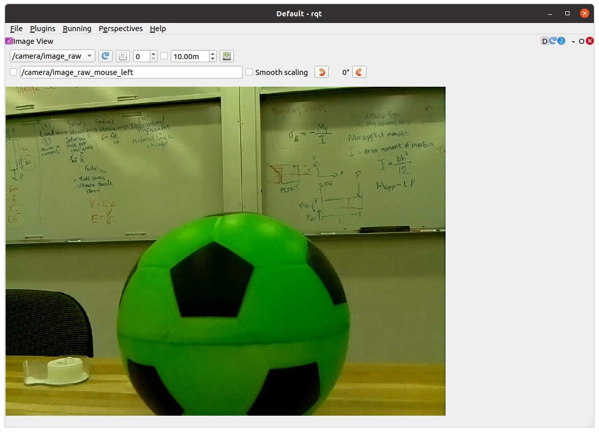
You can visualize the images coming from the camera using rqt. First launch rqt.
$ rqt
Next, go to Plugins, then Visualization, and then select Image View. Select /camera/image_raw from the drop down menu. If you did this properly you should see the following on your screen.
Run the starter code and you’ll see the dimensionality of the resultant numpy array as printed out in process_image. You’ll notice that the encoding of the image is bgr8 which means that the color channels of the 1024x768 image are stored in the order blue first, then green, then red. Each color intensity is an 8-bit value ranging from 0-255.
If all went well, you should see an image pop up on the screen that shows both the raw camera feed as well as a color filtered version of the image.
Note: a very easy bug to introduce into your opencv code is to omit the call to the function
cv2.waitKey(5). This function gives the OpenCV GUI time to process some basic events (such as handling mouse clicks and showing windows). If you remove this function from the code above, check out what happens.
Do some filtering based on color
The color filtering image is produced sing the cv2.inRange function to create a binarized version of the image (meaning all pixels are either black or white) depending on whether they fall into the specified range. As an example, here is the code that creates a binary image where white pixels would correspond to brighter pixels in the original image, and black pixels would correspond to darker ones
self.binary_image = cv2.inRange(self.cv_image, (128,128,128), (255,255,255))
This code could be placed inside of the process_image function at any point after the creation of self.cv_image. Notice that there are three pairs lower and upper bounds. Each pair specifies the desired range for one of the color channels (remember, the order is blue, green, red). If you are unfamiliar with the concept of a colorspaces, you might want to do some reading about them on Wikipedia. Here is the link to the RGB color space (notice the different order of the color channels from OpenCV’s BGR). Another website that might be useful is this color picker widget that lets you see the connection between specific colors and their RGB values.
Your next goal is to choose a range of values that can successfully locate the ball. In order to see if your binary_image successfully segments the ball from other pixels, you should visualize the resultant image using the cv2.namedWindow (for compatibility with later sample code you should name your window binary_image) and cv2.imshow commands (these are already in the file, but you should use them to show your binarized image as well).
Super, super, super important: any interaction with opencv’s GUI functios (e.g.,
cv2.namedWindoworcv2.imshow) should only be done inside ofloop_wrapperorrun_loopfunctions (this is because you want to interact with the UI of OpenCV from the same thread).
Also important: white pixels will correspond to pixels that are in the specified range and black pixels will correspond to pixels that are not in the range (it’s easy to convince yourself that it is the other way around, so be careful).
Debugging Tips
We have added some code so that when you hover over a particular pixel in the image we display the r, g, b values. If you are curious, we do that using the following line of code.
cv2.setMouseCallback('video_window', self.process_mouse_event)
We then added the following mouse callback function.
    def process_mouse_event(self, event, x,y,flags,param):
        """ Process mouse events so that you can see the color values
            associated with a particular pixel in the camera images """
        image_info_window = 255*np.ones((500,500,3))
        cv2.putText(image_info_window,
                    'Color (b=%d,g=%d,r=%d)' % (self.cv_image[y,x,0], self.cv_image[y,x,1], self.cv_image[y,x,2]),
                    (5,50),
                    cv2.FONT_HERSHEY_SIMPLEX,
                    1,
                    (0,0,0))
A second debugging tip is to use sliders to set your lower and upper bounds interactively. In this page, I’ll walk you through adding these using OpenCV, but you could also use dynamic_reconfigure (e.g., see this example from Day 4 of class).
To get started I’ll walk you through making the lower bound for the red channel configurable using a slider. First, add these lines of code to your loop_wrapper function. This code will create a class attribute to hold the lower bound for the red channel, create the thresholded window, and add a slider bar that can be used to adjust the value for the lower bound of the red channel.
        cv2.namedWindow('binary_image')
        self.red_lower_bound = 0
        cv2.createTrackbar('red lower bound', 'binary_window', self.red_lower_bound, 255, self.set_red_lower_bound)
The last line of code registers a callback function to handle changes in the value of the slider (this is very similar to handling new messages from a ROS topic). To create the call back, use the following code:
    def set_red_lower_bound(self, val):
        """ A callback function to handle the OpenCV slider to select the red lower bound """

        self.red_lower_bound = val
All that remains is to modify your call to the inRange function to use the attribute you have created to track the lower bound for the red channel. Remember the channel ordering!!! In order to fully take advantage of this debugging approach you will want to create sliders for the upper and lower bounds of all three color channels.
Here is what the UI will look like if you add support for these sliders.
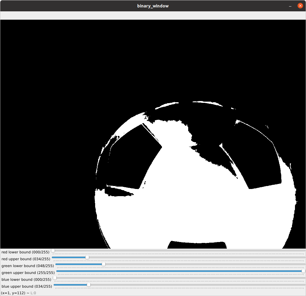
The code that generated this visual is included in the neato_soccer package as ball_tracker_solution.py. You can run it through the following command.
$ ros2 run neato_soccer ball_tracker_solution
If you find the video feed lagging on your robot, it may be because your code is not processing frames quickly enough. Try only processing every fifth frame to make sure your computer is able to keep up with the flow of data.
An Alternate Colorspace
Separating colors in the BGR space can be difficult. To best track the ball, I recommend using the hue, saturation, value (or HSV) color space. See the Wikipedia page for more information. One of the nice features of this color space is that hue roughly corresponds to what we might color while the S and the V are aspects of that color. You can make a pretty good color tracker by narrowing down over a range of hues while allowing most values of S and V through (at least this worked well for me with the red ball).
To convert your RGB image to HSV, all you need to do is add this line of code to your process_image function.
self.hsv_image = cv2.cvtColor(self.cv_image, cv2.COLOR_BGR2HSV)
Once you make this conversion, you can use the inRange function the same way you did with the BGR colorspace. You may want to create two binarized images that are displayed in two different windows (each with accompanying sliders bars) so that you can see which works better.
Dribbling the Ball
There are probably lots of good methods, but what we implemented was basic proportional control using the center of mass in the x-direction of the binarized image. If the center of mass was in the middle 50% of the image we kept moving forward at a constant rate, if not, we rotated in place in order to move the ball into the middle 50% before moving forward again.
Tips:
- To compute the center of mass in the x-direction, use the ``cv2.moments`` function. Take a second to pull up the documentation for this function and see if you can understand what the code below is doing. You can easily code this in pure Python, but it will be pretty slow. For example, you could add the following code to your process_image function.
moments = cv2.moments(self.binary_image) if moments['m00'] != 0: self.center_x, self.center_y = moments['m10']/moments['m00'], moments['m01']/moments['m00'] -
When doing your proportional control, make sure to normalize self.center_x based on how wide the image is. Specifically, you'll find it easier to write your proportional control if you rescale self.center_x to range from -0.5 to 0.5. We recommend sending the motor commands in the self.run function.
If you want to use the sliders to choose the right upper and lower bounds before you start moving, you can set a flag in your __init__ function that will control whether the robot should move or remain stationary. You can toggle the flag in your process_mouse_event function whenever the event is a left mouse click. For instance if your flag controlling movement is should_move you can add this to your process_mouse_event function:
        if event == cv2.EVENT_LBUTTONDOWN:
            self.should_move = not(self.should_move)